

推荐引擎是使浏览内容更容易的强大工具。此外,一个出色的推荐系统可以帮助用户找到他们自己不会想到要寻找的东西。由于这些原因,推荐工具可以极大地提高电子商务的营业额。在这里,我们展示了我们如何 - 在法国迪卡侬 - 实现了一个 RNN(循环神经网络)推荐系统,该系统在精度指标(离线)上比我们之前的模型(ALS,交替最小二乘法)高出 20% 以上。
如果您正在寻找有关推荐系统的更全面介绍,我们建议您阅读我们加拿大同事的精彩文章。
业务问题
迪卡侬在线目录非常大,我们在我们的在线平台上销售数万种不同的商品。对于寻找引人注目的新内容的用户来说,如此广泛的选择可能是一个障碍。当然,客户可以使用搜索来访问内容。在这方面,推荐引擎可以派上用场,因为它可以显示用户可能不会自己搜索的项目,从而极大地提高客户体验和转化率。
为了改进我们之前的解决方案 (ALS),我们开发了一个新的推荐引擎(基于深度学习),为每个确定的客户个性化 www.decathlon.fr 的主页。因此,每个识别出的用户都会看到不同的个性化推荐。
数据科学解决方案
我们之前的推荐系统是使用 spark.ml 库实现的协同过滤。 spark.ml 包使用交替最小二乘 (ALS) 算法来学习用户-项目关联矩阵的潜在因素。
协同过滤通常用于推荐系统。然而,事实证明它是一个严格的框架,阻止使用任何其他有用的元数据。此外,它假设用户和项目仅线性相关。最近的工作(Netflix、YouTube、Spotify)表明,由于使用了更丰富的输入数据非线性变换以及添加了有用的元数据,深度学习框架的性能优于经典分解方法。
我们的深度学习方法受到最近的文本生成技术的启发,这些技术使用能够从给定短语(单词序列)生成后续单词的 RNN 模型。对于我们的推荐问题,我们用项目序列替换了词序列并应用了相同的方法(下图描述了 NLP 和推荐的类比)。
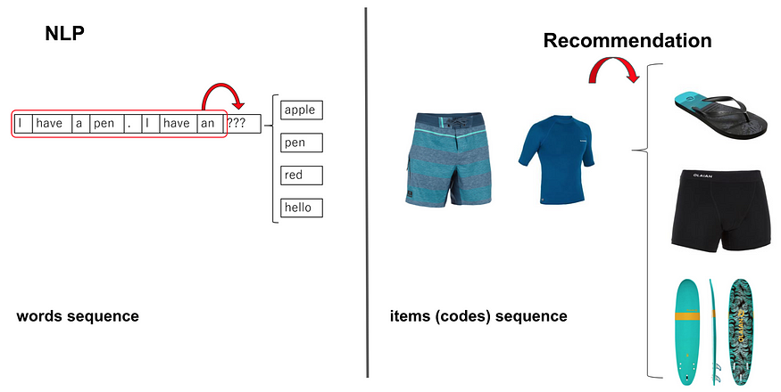
NLP and Recommandation analogy to predict the next more likely word and item respectively
输入数据
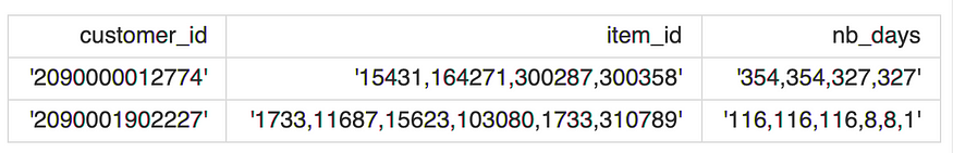
用于开发我们的推荐引擎的数据包括每个已识别客户的购买商品的时间排序序列和(购买商品的)新近度序列。 这是我们输入数据的示例:
在哪里:
- customer_id :是客户唯一标识符;
- item_id :包含每个客户购买的商品 ID 序列的字符串;
- nb_days:包含从物品购买和上次培训日期(每件购买物品的购买新近度)经过的天数序列的字符串。
注意:item_id 和 nb_days 序列是按时间顺序排列的。
特征变换
特征 item_id 和 nb_days 在将它们提供给模型之前需要适当地转换。即,item_id 将被标记和编码,而 nb_days 将被分桶。
item_id 的标记化和编码
为了为 RNN 模型准备输入数据,每个购买的商品序列都被标记化,并且序列中的每个商品都被整数编码。
这是通过使用 tensorflow.keras.preprocessing.text 中的 Tokenizer 类实现的,该类允许向量化文本语料库,通过将每个文本转换为整数序列(查看文档了解更多详细信息)。比如上面的item序列的字符串变成了下面的数组(numpy):
"15431,164271,300287,300358"->[74, 276, 362, 119]"1733,11687,15623,103080,1733,310789"->[1, 2, 33, 289, 1, 27].
nb_days 的分桶
nb_days 特征包含从 365 到 1 的整数值的可变长度序列。这是因为我们提取了一年的交易历史,因此 365 表示购买商品的最旧时间(以天表示的一年),1 表示最近一次。
我们决定将 nb_days 分成 100 个 bins(如果需要,这个值可以改变),用 1 到 100 的离散值表示。例如,上面的新近序列字符串变成以下数组(numpy):
'354,354,327,327'->[96, 96, 89, 89]'116,116,116,8,8,1'->[32, 32, 32, 2, 2, 1].
这种转换可以通过 tensorflow.feature_column.bucketized_column 轻松实现。
创建输入和目标特征张量
为了训练模型,我们需要创建一个包含输入和目标特征的张量。
值得注意的是,输入特征是 item_id 和 nb_days 的转换版本,没有最后一个元素,而目标特征是 item_id 的转换版本(没有第一个元素)。
这是因为我们想让 RNN 模型学习在给定先前输入特征的情况下预测目标序列的下一项。
例如,如果 item_id、nb_days 的变换特征分别为 [74, 276, 362, 119] 和 [96, 96, 89, 89],则特征张量将为:
{
'item_id': [74, 276, 362],
'nb_days': [96, 96, 89],
'target': [276, 362, 119]
}
填充
为了使所有序列的长度相同,然后通过 tensorflow.keras.preprocessing.sequence 中的 pad_sequences() 函数填充输入和目标特征。为了我们的目的,我们发现将每个序列的最大长度固定为 20(max_len,程序配置的一部分)工作正常。该值对应于序列长度的第 80 个百分位,即 80% 的 item_id 序列由最多 20 个项目组成。
例如,当 max_len = 5 时,上例的特征张量将变为:
{
'item_id': [0, 0, 74, 276, 362],
'nb_days': [0, 0, 96, 96, 89],
'target': [0, 0, 276, 362, 119]
}
特征数据
最终的特征数据是一个字典,其键是 item_id、nb_days、target,值是 N x max_length numpy 数组,其中 N 表示用于训练的序列数(最多为用户数),max_length 是用于填充的最大长度.
train_dict = {
              'item_id': [[0, 0,...,0, 74, 276, 362], ...]
              'nb_days': [[0, 0,...,0, 96, 96, 89], ...]
              'target':  [[0, 0,...0, 276, 362, 119], ...]
             }
最终,我们使用 tf.data.Dataset.from_tensor_slices 函数创建了一个用于模型训练的训练数据集(见下面的代码)。
import tensorflow as tf

def create_train_tfdata(train_feat_dict, train_target_tensor,
                        batch_size, buffer_size=None):
    """
    Create train tf dataset for model train input
    :param train_feat_dict: dict, containing the features tensors for train data
    :param train_target_tensor: np.array(), the training TARGET tensor
    :param batch_size: (int) size of the batch to work with
    :param buffer_size: (int) Optional. Default is None. Size of the buffer
    :return: (tuple) 1st element is the training dataset,
                     2nd is the number of steps per epoch (based on batch size)
    """
    if buffer_size is None:
        buffer_size = batch_size*50

    train_steps_per_epoch = len(train_target_tensor) // batch_size

    train_dataset = tf.data.Dataset.from_tensor_slices((train_feat_dict,
                                                        train_target_tensor)).cache()
    train_dataset = train_dataset.shuffle(buffer_size).batch(batch_size)
    train_dataset = train_dataset.repeat().prefetch(tf.data.experimental.AUTOTUNE)

    return train_dataset, train_steps_per_epoch

  train_feat_dict = {'item_id': train_dict['item_id'],
                     'nb_days': train_dict['nb_days']}
  train_target_tensor = train_dict['target']

  train_dataset, train_steps_per_epoch = create_train_tfdata(train_feat_dict,
                                                             train_target_tensor,
                                                             batch_size=512)
模型
此处实施的建模策略包括根据之前购买的商品的顺序(item_id 功能)和购买新近度(nb_days 功能)为每个用户预测下一个最有可能购买的产品。
nb_days 功能在显着提高模型性能方面发挥了关键作用。 事实上,此功能有助于模型更好地跟踪购买的季节性行为,从而跨时间推荐更适合的产品。
最后,我们还添加了一个自我注意层,它已被确定为序列到序列模型架构的性能助推器,就像我们的例子一样。
因此,这里实现的模型是一个 RNN 模型,加上一个具有以下架构的自注意力层:

Recommendation Engine model architecture
模型的超参数为:
- emb_item_id_units:每个项目(item_id)将被编码(嵌入)在一个形状为(1,emb_item_id_units)的密集向量中
- emb_nb_days_units:每个分桶的新近值 (nb_days) 将被编码(嵌入)在一个形状为 (1, emb_nb_days_units) 的密集向量中
- recurrent_dropout:LSTM 层的 drop-out 值
- rnn_units:LSTM 层的单元(“神经元”)数量
- learning_rate: 训练模型的学习率
而(不可调整的)参数是:
- max_length:每个item序列的最大长度,见数据预处理部分
- item_id_vocab_size:唯一项的数量 + 1(考虑到零填充)
- batch_size:同时提供给模型进行训练的样本(序列)数量
在这里你可以找到上述推荐架构的 TensorFlow 实现:
def build_model(hp, max_len, item_vocab_size):
    """
    Build a model given the hyper-parameters with item and nb_days input features
    :param hp: (kt.HyperParameters) hyper-parameters to use when building this model
    :return: built and compiled tensorflow model
    """
    inputs = {}
    inputs['item_id'] = tf.keras.Input(batch_input_shape=[None, max_len],
                                       name='item_id', dtype=tf.int32)
    # create encoding padding mask
    encoding_padding_mask = tf.math.logical_not(tf.math.equal(inputs['item_id'], 0))

    # nb_days bucketized
    inputs['nb_days'] = tf.keras.Input(batch_input_shape=[None, max_len],
                                       name='nb_days', dtype=tf.int32)

    # Pass categorical input through embedding layer
    # with size equals to tokenizer vocabulary size
    # Remember that vocab_size is len of item tokenizer + 1
    # (for the padding '0' value)

    embedding_item = tf.keras.layers.Embedding(input_dim=item_vocab_size,
                                               output_dim=hp.get('embedding_item'),
                                               name='embedding_item'
                                              )(inputs['item_id'])
    # nbins=100, +1 for zero padding
    embedding_nb_days = tf.keras.layers.Embedding(input_dim=100 + 1,
                                                  output_dim=hp.get('embedding_nb_days'),
                                                  name='embedding_nb_days'
                                                 )(inputs['nb_days'])

    #  Concatenate embedding layers
    concat_embedding_input = tf.keras.layers.Concatenate(
     name='concat_embedding_input')([embedding_item, embedding_nb_days])

    concat_embedding_input = tf.keras.layers.BatchNormalization(
     name='batchnorm_inputs')(concat_embedding_input)

    # LSTM layer
    rnn = tf.keras.layers.LSTM(units=hp.get('rnn_units_cat'),
                                   return_sequences=True,
                                   stateful=False,
                                   recurrent_initializer='glorot_normal',
                                   name='LSTM_cat'
                                   )(concat_embedding_input)

    rnn = tf.keras.layers.BatchNormalization(name='batchnorm_lstm')(rnn)

    # Self attention so key=value in inputs
    att = tf.keras.layers.Attention(use_scale=False, causal=True,
                                    name='attention')(inputs=[rnn, rnn],
                                                      mask=[encoding_padding_mask,
                                                            encoding_padding_mask])

    # Last layer is a fully connected one
    output = tf.keras.layers.Dense(item_vocab_size, name='output')(att)

    model = tf.keras.Model(inputs, output)

    model.compile(
        optimizer=tf.keras.optimizers.Adam(hp.get('learning_rate')),
        loss=loss_function,
        metrics=['sparse_categorical_accuracy'])

    return model
TensorFlow implementation of the RNN recommendation engine
作为损失函数,我们使用了 tf.keras.losses.sparse_categorical_crossentropy 的修改版本,其中我们跳过了零填充元素的损失计算:
def loss_function(real, pred):
    """
    We redefine our own loss function in order to get rid of the '0' value
    which is the one used for padding. This to avoid that the model optimize itself
    by predicting this value because it is the padding one.

    :param real: the truth
    :param pred: predictions
    :return: a masked loss where '0' in real (due to padding)
                are not taken into account for the evaluation
    """

    # to check that pred is numric and not nan
    mask = tf.math.logical_not(tf.math.equal(real, 0))
    loss_object_ = tf.keras.losses.SparseCategoricalCrossentropy(from_logits=True,
                                                                 reduction='none')
    loss_ = loss_object_(real, pred)
    mask = tf.cast(mask, dtype=loss_.dtype)
    loss_ *= mask

    return tf.reduce_mean(loss_)
TensorFlow implementation of custom loss function
超参数优化
模型超参数已经使用在 keras-tuner 库中实现的 Hyperband 优化算法进行了调整,这使得人们可以用几行代码为 TensorFlow 模型进行可分发的超参数优化
值得注意的是,超参数优化是使用验证数据集进行的,该数据集由训练数据中随机选择的样本的 10% 组成。 此外,我们使用 sparse_categorical_accuracy 作为衡量优化试验排名的指标。
我们为batch_size 参数尝试了几个值,最终使用batch_size=512。
训练
最终模型在所有可用数据上进行训练,并使用在前一个优化阶段结束时获得的最佳超参数进行训练。
def fit_model(model, train_dataset, steps_per_epoch, epochs):
    """
    Fit the Keras model on the training dataset for a number of given epochs
    :param model: tf model to be trained
    :param train_dataset: (tf.data.Dataset object) the training dataset
                          used to fit the model
    :param steps_per_epoch: (int) Total number of steps (batches of samples) before
                            declaring one epoch finished and starting the next epoch.
    :param epochs: (int) the number of epochs for the fitting phase
    :return: tuple (mirrored_model, history) with trained model and model history
    """

    # mirrored_strategy allows to use multi GPUs when available
    mirrored_strategy = tf.distribute.experimental.MultiWorkerMirroredStrategy(
        tf.distribute.experimental.CollectiveCommunication.AUTO)

    with mirrored_strategy.scope():
        mirrored_model = model

    history = mirrored_model.fit(train_dataset,
                                 steps_per_epoch=steps_per_epoch,
                                 epochs=epochs, verbose=2)

    return mirrored_model, history
TensorFlow implementation of the fitting method
结果
在使用我们的新推荐系统之前,我们采用了回测策略来评估模型预测性能。 事实上,回溯测试通过发现模型如何使用历史数据进行回顾来评估模型的可行性。
其基本理论是,任何过去运行良好的模型将来都可能运行良好,反之,任何过去运行不佳的模型在未来都可能运行不佳。
为此,我们使用了一年的历史交易作为训练数据,并在接下来的一个月测试了模型性能(见下图)。
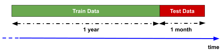
Backtesting strategy representation
下表显示了几个模型在回测期间的基准性能。 我们使用经典指标对推荐模型的结果进行排名,即精度、召回率、MRR、MAP 和覆盖率,所有这些指标都是根据每个用户最好的五个推荐项目计算的。

Benchmark of backtesting results (orange-production, green-challenger, gray-baseline)
橙色线代表实际生产模型 (ALS) 性能,这是我们旨在改进的性能。我们开发了多个版本的 RNN 推荐系统(挑战者、绿线),其复杂程度不断提高。
最简单的 RNN,仅包含 item_id 作为特征,接近 ALS 性能,但在几乎所有指标上都较差。
最大的改进提升是由于添加了 nb_days 功能。这种时间特征允许基于 RNN 的推荐系统在所有给定指标上明显超越 ALS 模型。最后,注意力层的加入最终提高了 RNN 的整体性能。
为了可比性,我们还计算了一些(简单的)基线(表中的灰色线),它们清楚地显示了与更复杂模型(ALS 和 RNN 版本)的性能差距。
在线 A/B 测试正在进行中,初步结果证实了 RNN 推荐引擎的卓越性能。
结论
我们已经描述了我们用于在迪卡侬网站上推荐项目的新深度神经网络架构,并展示了如何使用 TensorFlow 实现它。该模型 - 受最近的文本再生技术启发 - 使用循环神经网络 (RNN) 架构,其输入是与购买新近序列(nb_days 功能)相关联的已购买商品序列。由于深度学习模型需要输入特征的特殊表示,我们还描述了如何在将这些输入序列(item_id 和 nb_days)馈送到模型之前正确转换它们。
最后,通过回测策略,我们展示了 nb_days 特征的使用如何在超越我们基于矩阵分解方法 (ALS) 的历史生产模型方面发挥关键作用。
这种新的深度学习架构为我们提供了添加新功能(与用户和项目相关)的可能性,从而可以进一步提高模型性能和用户体验,从而开辟了新的视角。
你呢? 您在深度学习和推荐系统方面有经验吗? 请在下面的评论中告诉我们!
原文:https://medium.com/decathlontechnology/building-a-rnn-recommendation-en…